Using statsmodels for Regression

In the previous section, we used functions in NumPy and concepts taught in Data 8 to perform single variable regressions. It turns out that there are (several) Python packages that can perform these regressions for us and which extend nicely into the types of regressions we will cover in the next few sections. In this section, we introduce statsmodels for performing single variable regressions, a foundation upon which we will build our discussion of multivariable regression.

statsmodels is a popular Python package used to create and analyze various statistical models. To create a linear regression model in statsmodels, which is generally import as sm, we use the following skeleton code:

x = data.select(features).values            # Separate features (independent variables) 
y = data.select(target).values              # Separate target (outcome variable)
model = sm.OLS(y, sm.add_constant(x))       # Initialize the OLS regression model
result = model.fit()                        # Fit the regression model and save it to a variable
result.summary()                            # Display a summary of results

You must manually add a constant column of all 1’s to your independent features. statsmodels will not do this for you and if you fail to do this you will perform a regression without an intercept $\alpha$ term. This is performed in the third line by calling sm.add_constant on x. Also note that we call .values after we select the columns in x and y; this gives us NumPy arrays containing the corresponding values, since statsmodels can’t process Tables.

Recall the cps dataset we used in the previous section:

Let’s use statsmodels to perform our regression of logwage on educ again.

The summary above provides us with a lot of information. Let’s start with the most important pieces: the values of $\hat{\alpha}$ and $\hat{\beta}$. The middle table contains these values for us as const and x1’s coef values: we have $\hat{\alpha}$ is 1.4723 and $\hat{\beta}$ is 0.1078.

Recall also our discussion of uncertainty in $\hat{\beta}$. statsmodels provides us with our calculated standard error in the std err column, and we see that the standard error of $\hat{\beta}$ is 0.001, matching our empirical estimate via bootstrapping from the last section. We can also see the 95% confidence interval that we calculated in the two rightmost columns.

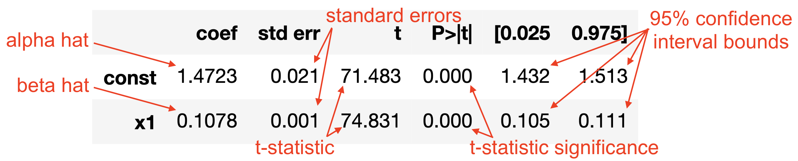
Earlier we said that $\hat{\beta}$ has some normal distribution with mean $\beta$ if certain assumptions are satisfied. We now can see that the standard deviation of that normal distribution is the standard error of $\hat{\beta}$. We can also use this to test a null hypothesis that $\beta = 0$. To do so, construct a t-statistic (which statsmodels does for you) that indicates how many standard deviations away $\hat{\beta}$ is from 0, assuming that the distribution of $\hat{\beta}$ is in fact centered at 0.

We can see that $\hat{\beta}$ is 74 standard deviations away from the null hypothesis mean of 0, which is an enormous number. How likely do you think it is to draw a random number roughly 74 standard deviations away from the mean, assuming a standard normal distribution? Essentially 0. This is strong evidence that the mean of the distribution (the mean of $\hat{\beta}$ is the true value $\beta$) is not 0. Accompanying the t-statistic is a p-value that indicates the statistical significance.